
Gradient Descent
After choosing a cost function you need to minimize that function to slow the error. How we do that? with gradient descendent. There are different methods to optimize the cost function. These methods are called optimization methods and all of them use a modification of gradient descend to get the minima(There are others, but they use second order derivates like Newton’s method). Each has evolved from previous methods of gradient descent to solve problems that overcome previews methods. Regular gradient descent can`t work with big DataSets because there’s, not enough memory for the large computational memory that gradient descent takes. Gradient descendant is a method that helps us find the minima of a function. Now you are asking why do we have to use gradient methods instead of just derivate the function and use analytic math to find the minima? well for very complex network this is not an option for several reasons, like very high computational costs, and because in real life the equation that we get to find the minima are very complex. That is why we use gradient descendant to find the minima.
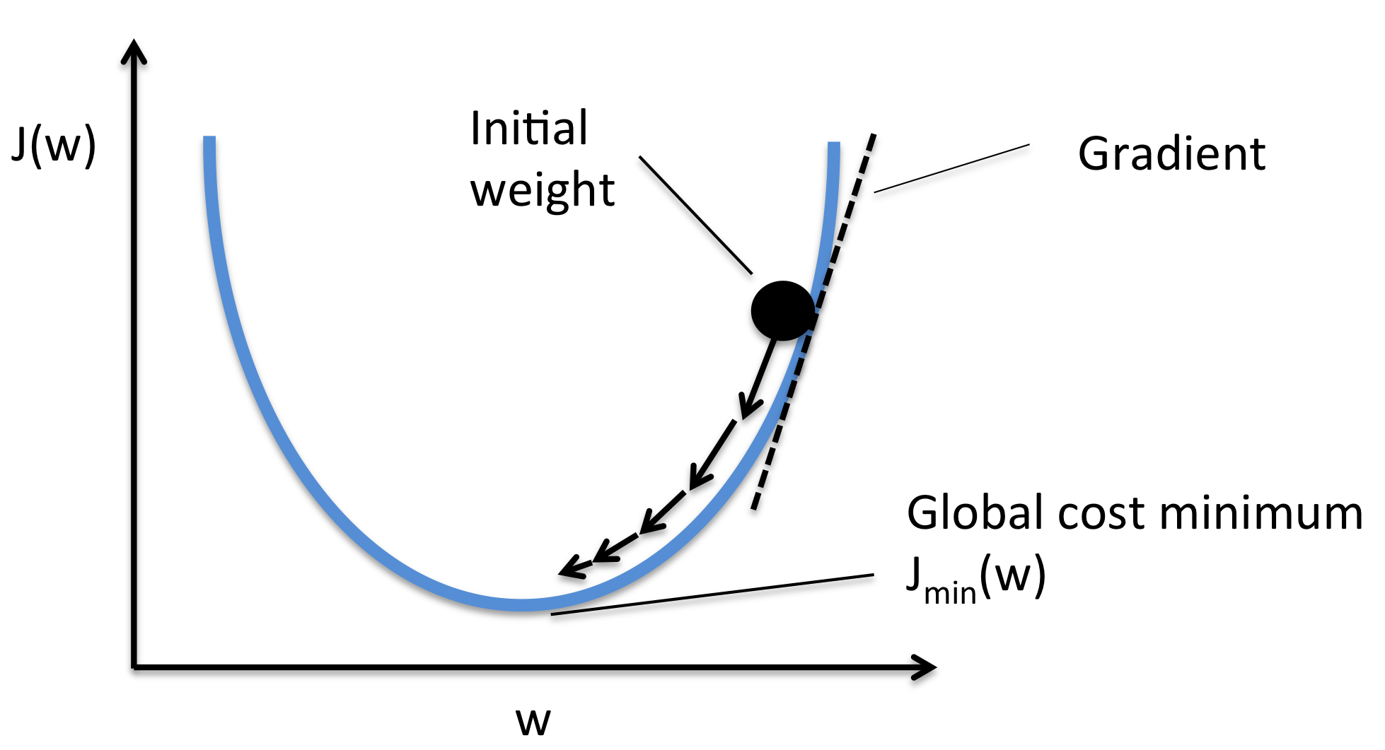
How Gradient Descent works
Gradient descent works by first choosing an arbitrary point and then taking small steps against the gradient by multiplying alpha (alpha is the small number for example 0.01) by the gradient until you get to the minima.
Gradient descent algorithm in python
min = 10
gamma = 0.01
presition = 0.0001
move = 1

#this is the derivate of the function x^2 - 6x
def derivate(x):
y = 2*x -6
return y

while move > presition:
gradient = function_derivate(min)
move = gamma * gradient
min = min - move

print("The minima is {}" .format(round(min,2)))
The problem with gradient descent is that we can get stuck in a local minimum when the function has 2 or more minimum. For that reason, we use stochastic gradient algorithm that behaves like a simulated annealing algorithm, where the learning rate of the SGD is related to the temperature of SA. The randomness or noise introduced by SG allows escaping from a local minimum to reach a better minimum.
If finding the global minimum is important then we can use a method such a simulated annealing. The problem with this methods is that they take a long time to find the global minimum.
But how important is to find the global minimum instead of a local minimum in a deep net? Well after reading this article it seems that finding global minima in deep nets appears to be unnecessary because the local minimum is approximately as good as the global minimum. More important is try to avoid over-fitting the neural network, if you aggressively searching for the global minimum of the cost function is likely to result in overfitting and a model will perform poorly.
Other Optimization Methods of Gradient Descent
Gradient descent is the foundation of how we train intelligent systems. Optimizations methods as Gradient Descent is what actually let our neural network learns from data. But gradient descent has a disadvantage with larger data sets because it gets slow. Gradient descent computes the gradient of the loss function base on the parameters of the entire training data set. As we need to calculate the gradient of the whole dataset for just update a single parameter it gets very slow. And with larger dataset, the memory can overflow. Stochastic Gradient Descent comes up to help us solve these problems.
Stochastic Gradient Descent
It also complicates the convergence because it can be overshooting. To solve this Mini-Batch Gradient Descent comes up.
Mini-Batch Gradient Descent
The isolation of MBGD makes it hard to converge, so a technique called momentum was invented to solve this problem
Momentum
Momentum is a method that helps accelerate SGD in the relevant direction and dampens oscillations. It does this by adding a fraction y of the update vector of the past time step to the current update vector. This means faster convergence and the reduced of Oscillations. But momentum has a problem, once we get near to the minimum the momentum is very high so it can miss the minima.
Nesterov Accelerated Gradient
Is the solution to solve that momentum miss the minima, it was called Nesterov for the inventor. (He also was the one who discovered the problem with the momentum). This solution prevents to go too fast to miss the minima.
AdaGrad (Adaptative Gradient)
It allows learning rate to adapt base on parameters.
At some points, the learning rates can get so small that the model stops learning. AdaDelta was invented to solve this problem.
AdaDelta
It prevents learning rate decay.
So what we have to now? Our improvements so far:
- Individual learning rates per parameter
- Calculating momentum values
- Preventing decaying learning rates
Adam (Adaptative Moment Estimation)
For each parameter, it calculates learning rates and calculates momentum changes.
Conclusion Gradient Descent
Adam usually outperforms the rest of the optimizations methods. Followed by AdaGrad and AdaDelta.
For the other optimizations methods as Momentum, SGD and Nesterov they don´t perform well with datasets which data is sparse, and real life data sets the data are always sparse.
There also exists other algorithms to train neural networks like genetic algorithms, simulated annealing, and PSO. And theoretically, heuristic methods like Genetic algorithms and PSO are global optimizers. If you run them long enough they will find the global minimum. However, they would take much longer to converge to optimum compared to gradient descent. Also, genetic algorithms require a lot more sampling data, simulated annealing seems to deal with convergence in a one-form solution again and suffers by reducing the threshold cost allowed to travel to other permutation spaces until the model no longers updates and PSO depends on the topological initialization of the space.
As we have learned local minima works well enough and sometimes finding global minimums means overfitting our model.
Overfitting
In some point we have to introduce the problem of overfitting so, let’s talk about it. Overfitting is when your model performs very well with your training data but it performs badly with the test data. We say that the model has memorized the data and know very well how to react with the information that we just give them (training data) but it can`t generalize and it can`t give us good result with new data (test data).
But Overfitting always occurs?
I found this question and I would like to show it.
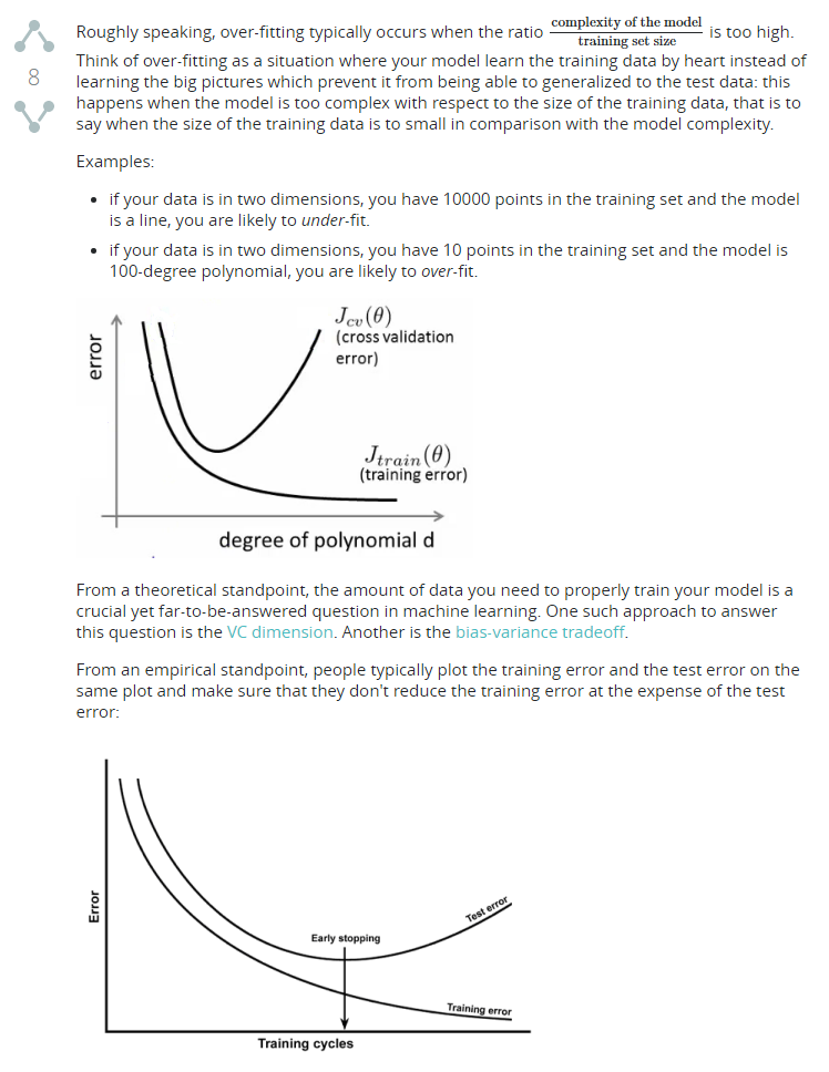
There are several ways of controlling the capacity of neural networks to prevent overfitting. Here I’m going to describe a resume. But you should read the Regularization part from CS231m
L2 regularization is perhaps the most common form of regularization. It can be implemented by penalizing the squared magnitude of all parameters directly in the objective.
L1 regularization is another relatively common form of regularization, where for each weight w we add the term λ∣w∣ to the objective.
Max norm constraints. Another form of regularization is to enforce an absolute upper bound on the magnitude of the weight vector for every neuron and use projected gradient descent to enforce the constraint.
Dropout is an extremely effective, simple and recently introduced regularization technique by Srivastava et al.
Batch Normalization: Reducing Internal Covariate Shift
Batch Normalization allows us to use much higher learning rates and be less careful about initialization. It also acts as a regularizer, in some cases eliminating the need for Dropout.
Vanishing gradient problem
Another problem we need to consider is Vanishing gradient problem.
Vanishing Gradient Problem is a difficulty found in training certain Artificial Neural Networks with gradient-based methods (e.g Back Propagation). In particular, this problem makes it really hard to learn and tune the parameters of the earlier layers in the network. This problem becomes worse as the number of layers in the architecture increases.
This is not a fundamental problem with neural networks – it’s a problem with gradient based learning methods caused by certain activation functions. Let’s try to intuitively understand the problem and the cause behind it.
The point of the paper is that when using random initialization one wants to pick the distribution for the random number generator carefully to avoid saturating the activation function at the next layer.
The vanishing gradient problem occurs because of the use of chain rule for backpropagation, and the fact that traditional activation functions (tanh and sigmoid ) produce values with magnitude less than 1(‘squash’ their input into a very small output range in a very non-linear fashion). As a result, there are large regions of the input space which are mapped to an extremely small range. In these regions of the input space, even a large change in the input will produce a small change in the output – hence the gradient is small.
But why to use a non-linear function like sigmoid functions in first place? Well, that is because without a non-linear function neural networks are only capable of modeling linear functions and as we know real world problems can be represented only as non-linear functions, so introducing non-linear functions allow neural networks to model real world problems.
So in a resume. By using activation functions the neural network is able to approximate non-linear functions (any process you can imagine can be thought as a non-linear computation function. ) So we add this activation function in order to make our neural network can model non-linear functions. If we didn´t add an activation function our model only would be able to compute linear functions.
So people use the following solutions:
- As Daniel Lindsäth has said, use ReLU neurons as activation function
- Combine careful initialization of weights (such that they are not initialized in the saturation region of the activation function) with small learning rates
- Batch Normalization, where they employ an adaptive and learned normalization scheme to force the activations of a layer the follow a single distribution, independent of the changes in the parameters of upstream layers (Accelerating Deep Network Training by Reducing Internal Covariate Shift)
The ReLU in action
If you consider a simple neural network whose error E depends on weight wij only through yj, where
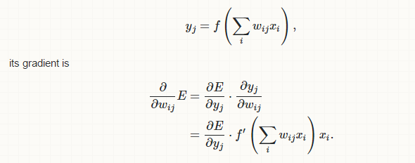
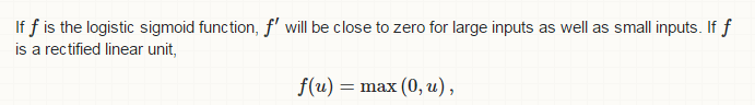
its gradient is zero only for negative inputs and large for large inputs.
Conclusion
We have learned what neural networks are for, the types of architectures and which one to chose depending on the problem. We’ve learned the problems that come up when training our neural network and what techniques, methods or solutions to use to avoid fall in those problems.
