
This is an extensive introduction, where we are going to know what are deep neural networks, we are going to know we mean when we talk about a feed forward neural network, what are they used for, when we use them either for classification or to make predictions, we are going to see that neural networks can solve non-linear problems. We are going to end up with the best approach for a feed forward neural network which is a neural network with only 2 or 3 hidden layers, that the activation function that best works are a Leaky RELU, that ADAMS is the best method for Stochastic Optimization which is the way that our neural networks learn base on our data.
In this blog, I am going to focus on Feed Forward Neural Network which is used to make classifications and predictions. It is used also in deep nets like convolutional neural networks as the final layer. It`s also important to know the different architectures for neural networks that exit. It is important because depending on the problem you want to solve you need to look for an architecture that is more suitable for solving a certain kind of problem.
Architectures of Deep Neural Networks
In the field of deep neural networks exits differents architectures, each architecture works better for certain kinds of problems. For example, Convolutional Neural Networks is a neural network architecture, it is used for visual classification and object detection.
Feed Fordward Neural Networks
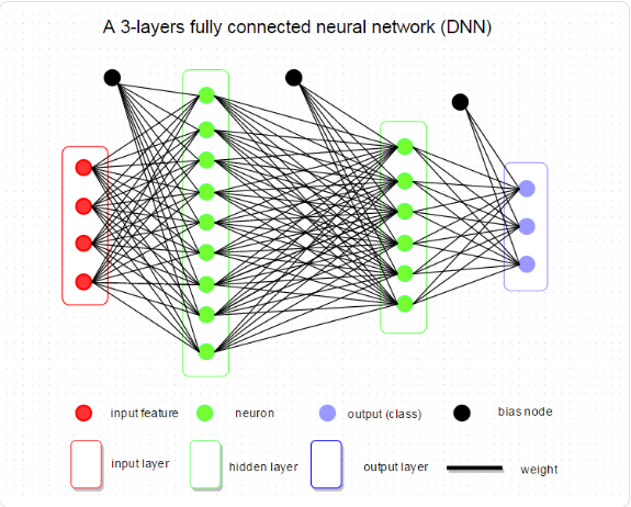
They are nodes grouped in rows and they are connected with each other between each row. Between each connection, there is a weigh that multiply the exit from the node with the weight and there is a bias that is summed.
This is the architecture.
And this is a closer neuron. In this example, the neuron only has one entry. This is just for an explanation. A real neuron can have multiples entries and each entry will have their own weight.
As you can see, the exit of this neuron will be the input multiplied by the weight plus the bias.
The next thing you need to know is that there is an activation function. There are a few activation functions for example, sigmoidal, tanh, reLu . Selecting one will change how the training of the network will change.
Vanishing gradient problem
Before continuing talking about the activation functions lets introduce the vanishing gradient problem. Vanishing Gradient Problem is a difficulty found in training certain Artificial Neural Networks with gradient based methods. In particular, this problem makes it really hard to learn and tune the parameters of the earlier layers in the network. This problem becomes worse as the number of layers in the architecture increases.This is not a fundamental problem with neural networks – it’s a problem with gradient based learning methods caused by certain activation functions. Vanishing gradient problem depends on the choice of the activation function. Many common activation functions (e.g sigmoid or tanh) ‘squash’ their input into a very small output range in a very non-linear fashion. We can avoid this problem by using activation functions which don’t have this property of ‘squashing’ the input space into a small region. A popular choice is Rectified Linear Unit which maps x to max(0,x). Find more details in here and the vanishing gradient problem in code. That is why the sigmoid function is rarely used in hidden layers.
So let’s go back to the neuron, as we can see the exit was equal to input*w + b. Ater that the exit is putting into an activation function and that is the actual output.
Now as I was saying this is just for explanation. A real neuron will have multiples entries.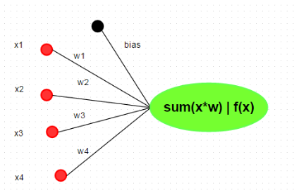
The output of that neuron will be:
Ok now that he have explained a little the architecture of a feedforward neural network, I’m going to explain about the input, the weights, and the outputs. I am going to explain that with an example that I heard. Suppose that you want to know if a married couple will divorce. The first thing you need is data and you make an investigation support that you interview 100 couple (In real life you will need more than that to training a neural network) with a question like:
- How many years do you live together before getting married?
- How many mts^2 was the house that you lived?
- How many windows your house had?
- How many kids did you have?
- How many rooms your house have?
- Finally, did you get divorced?
As you can see, a lot of question seem no having a sense of the context, but that is what is great about neural networks, they can find patterns where we can`t. All those data will be the input.
At first, the weights are a random number. When you introduce this inputs and multiply for the random weights this will produce also a random output. This will introduce us to supervised training (also exits unsupervised training and a combination of both). The supervised training is a classification for training data. It works by comparing the random output with the actual output given by the data we collected. This is how we can see the error to train the network until the error is minimum.
The example above guide us to the training step. The training step is where we modify the weights of our neural network to give us the desired output. To understand this step first you need to understand how we calculate the error. We need use a cost function, this cost function will tell us how far we are from the correct value. There are a lot of cost functions that we can use. The list below will show you the most used cost functions.
Here are those I understand so far. Most of these work best when given values between 0 and 1.
Quadratic cost
Also known as mean squared error, maximum likelihood, and sum squared error, this is defined as:
The gradient of this cost function with respect to the output of a neural network and some sample r is:
Cross-entropy cost
Also known as Bernoulli negative log-likelihood and Binary Cross-Entropy
The gradient of this cost function with respect to the output of a neural network and some sample r is:
Exponential cost
This requires choosing some parameter ττ that you think will give you the behavior you want. Typically you’ll just need to play with this until things work well.
Where simply shorthand for
.
The gradient of this cost function with respect to the output of a neural network and some sample r is:
I could rewrite out , but that seems redundant. The point is the gradient computes a vector and then multiplies it by
.
Hellinger distance
You can find more about this here. This needs to have positive values, and ideally values between 00and 11. The same is true for the following divergences.
The gradient of this cost function with respect to the output of a neural network and some sample r is:
Which cost function should I choose? Well, it depends. For example the Mean Square Error it`s a cost function that is used for regression (regression is used to predict values in the real space, and to predict stock houses prices or the large of an object in an image).
The Cross-Entropy it is a cost function that is used to feed a multinomial distribution and it is used to classified. What is does is to maximize the probability of an output given an input.
Both loss functions have explicit probabilistic interpretations. Square loss corresponds to estimating the mean of (any!) distribution. Cross-entropy with softmax corresponds to maximizing the likelihood of a multinomial distribution.
Intuitively, the square loss is bad for classification because the model needs the targets to hit specific values (0/1) rather than having larger values correspond to higher probabilities. This makes it really hard for the model to learn to express high and low confidence, and lots of times the model will struggle to keep values on 0/1 instead of doing something useful. (Reddit) Link.
